The inflatable curtain.
Sep 02, 2017
AirB'n'Berlin.
I. Definition
Project Overview
AirBnB is an online platform for accomodation. Since its launch in 2008, it provides now 3,000,000 lodging listings in 65,000 cities and 191 countries (source : wikipedia).
In Berlin, amongst the 17,810 registered hosts, 13% are considered as active users (the last review was done in the last 10 days). The first member registered in 2008, and there are 20,576 offers as of may 2017, 7700 being considered as active*.
In this study, we will focus on the full appartments offered on AirBnB in Europe, with a focus on Berlin.
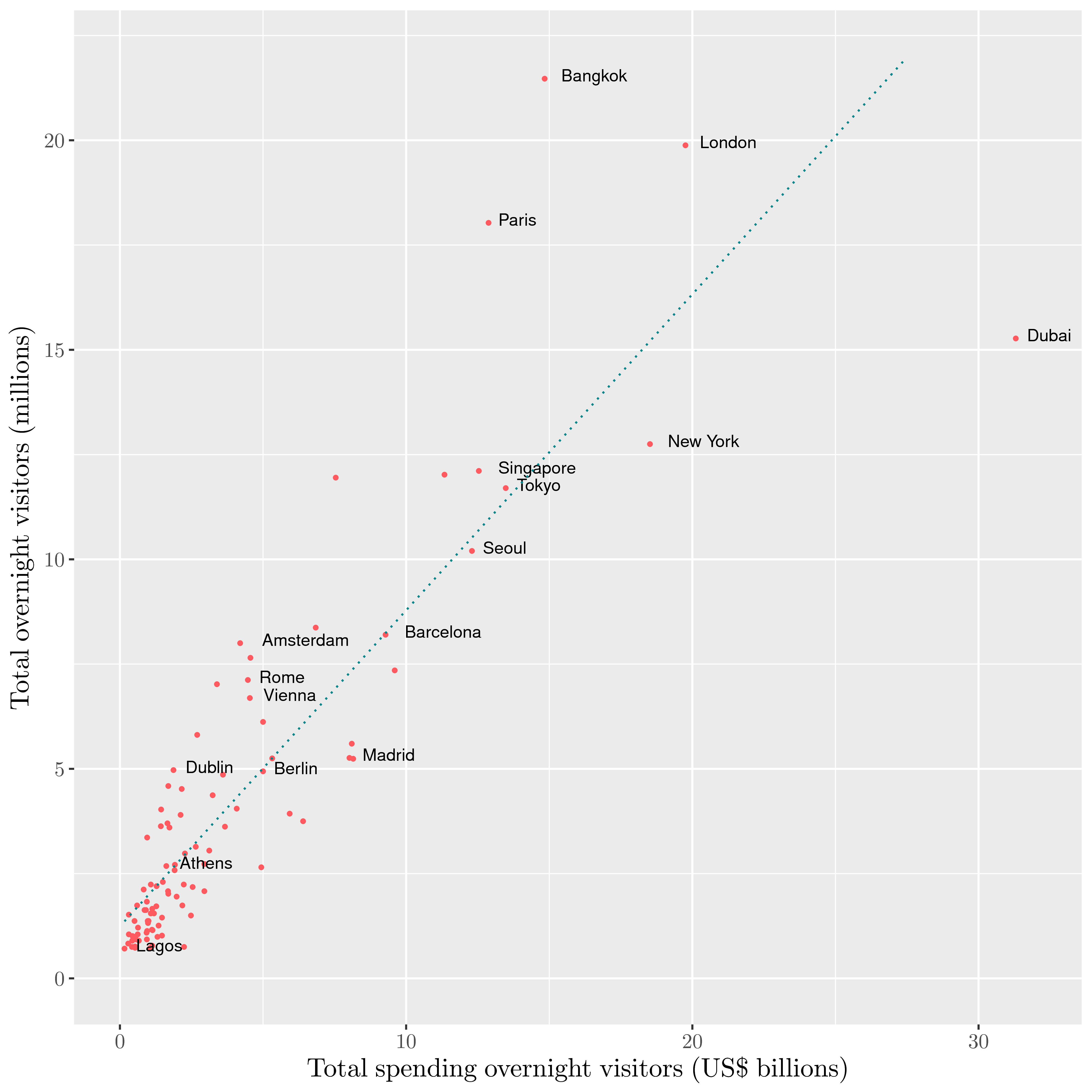
For the context, here are some charts to understand the situation of Berlin amongst the others world-class cities in term of tourism :
active listing : listing with an availability for the next 90 days higher than zero and with at least one review in the last 60 days.
| Visitors vs expenditures |
|---|
 |
| AirBnB renting structure |
|---|
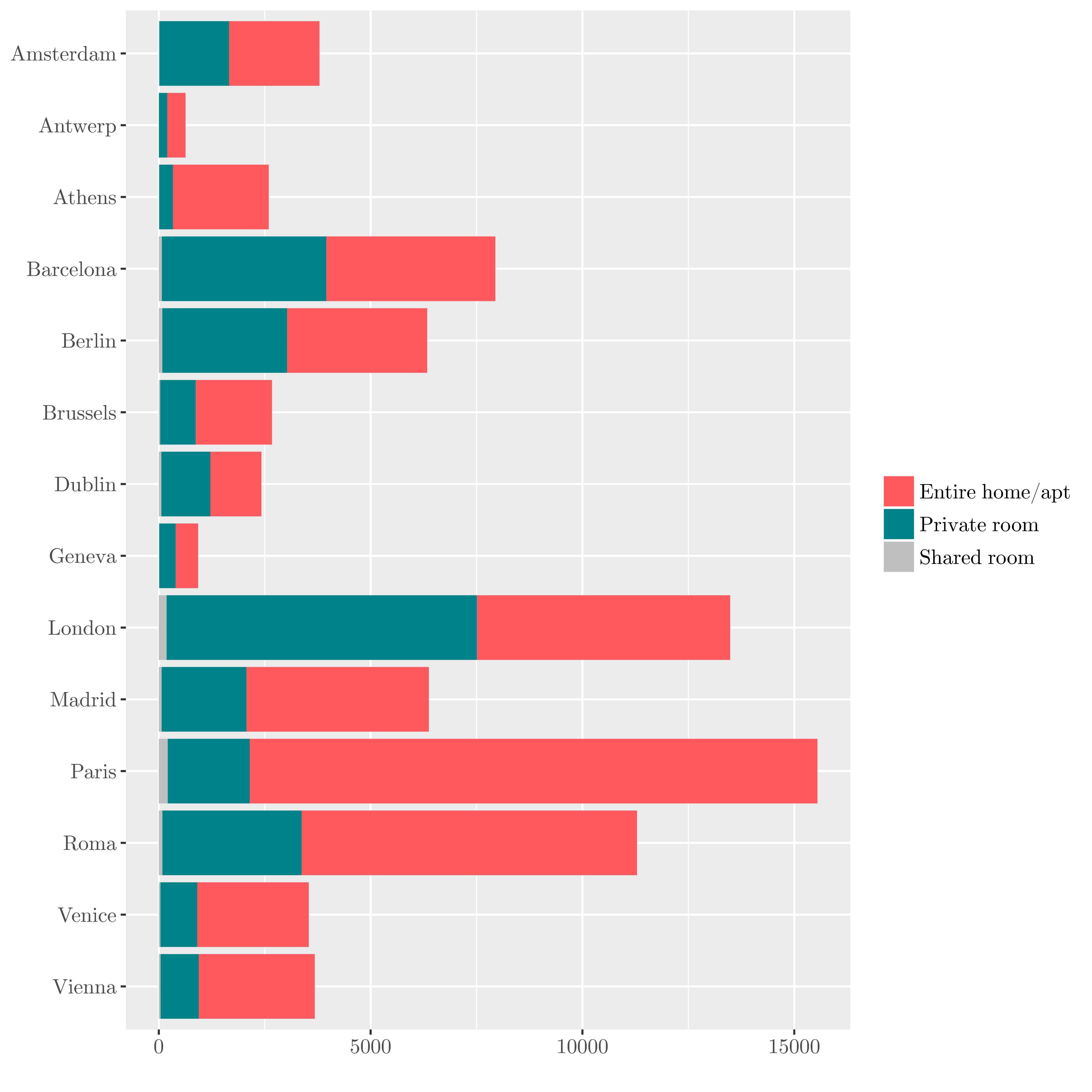 |
For a population of 3,5 Millions inhabitants, Berlin has a relatively low number of active offers compared to Amsterdam (population 0,85 Millions) or Barcelona (population 1,6 Millions).
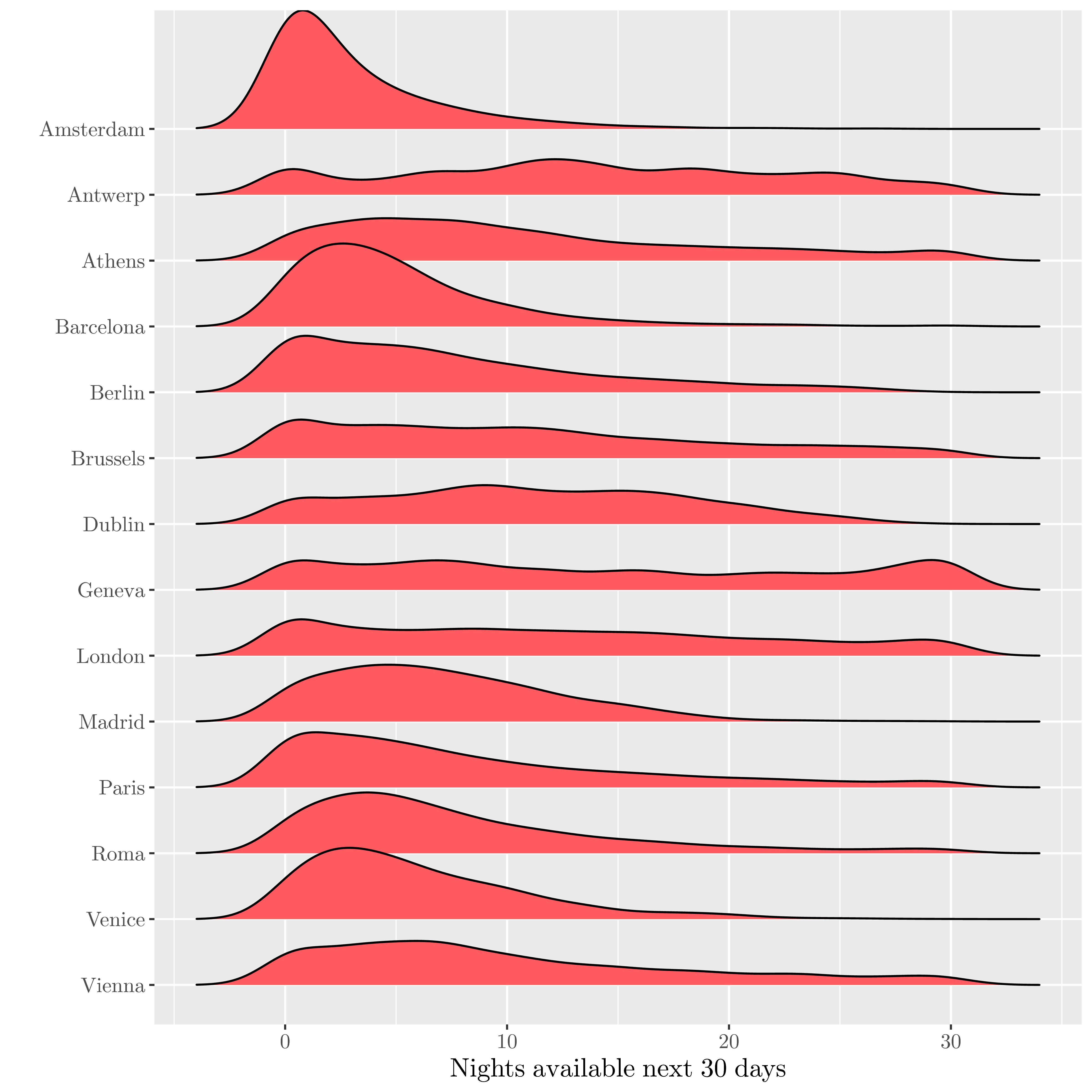
| Full appartments availability coming 30 days |
|---|
 |
| Full appartments prices |
|---|
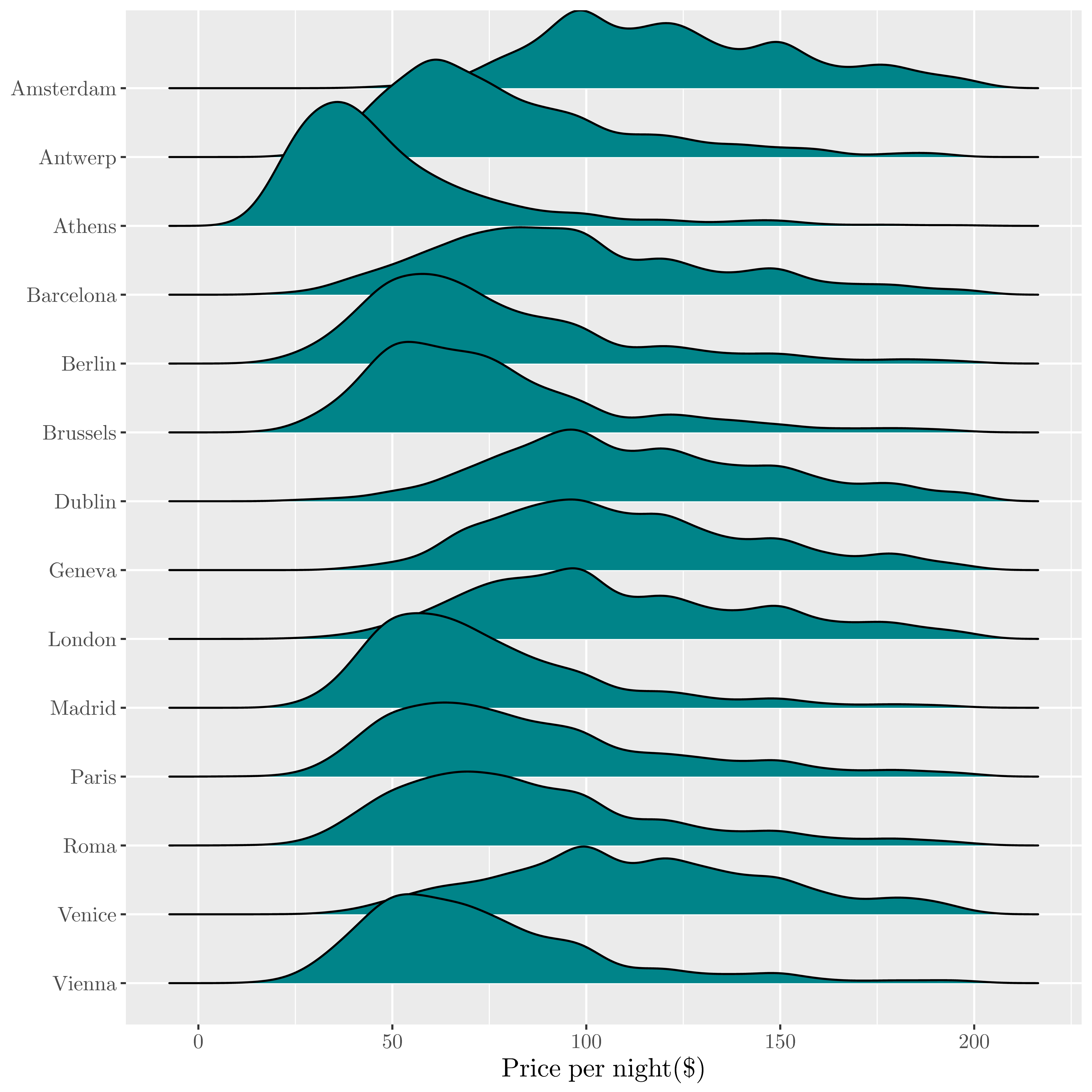 |
In term of price and availability, Berlin ranks in the average value on the european scale.
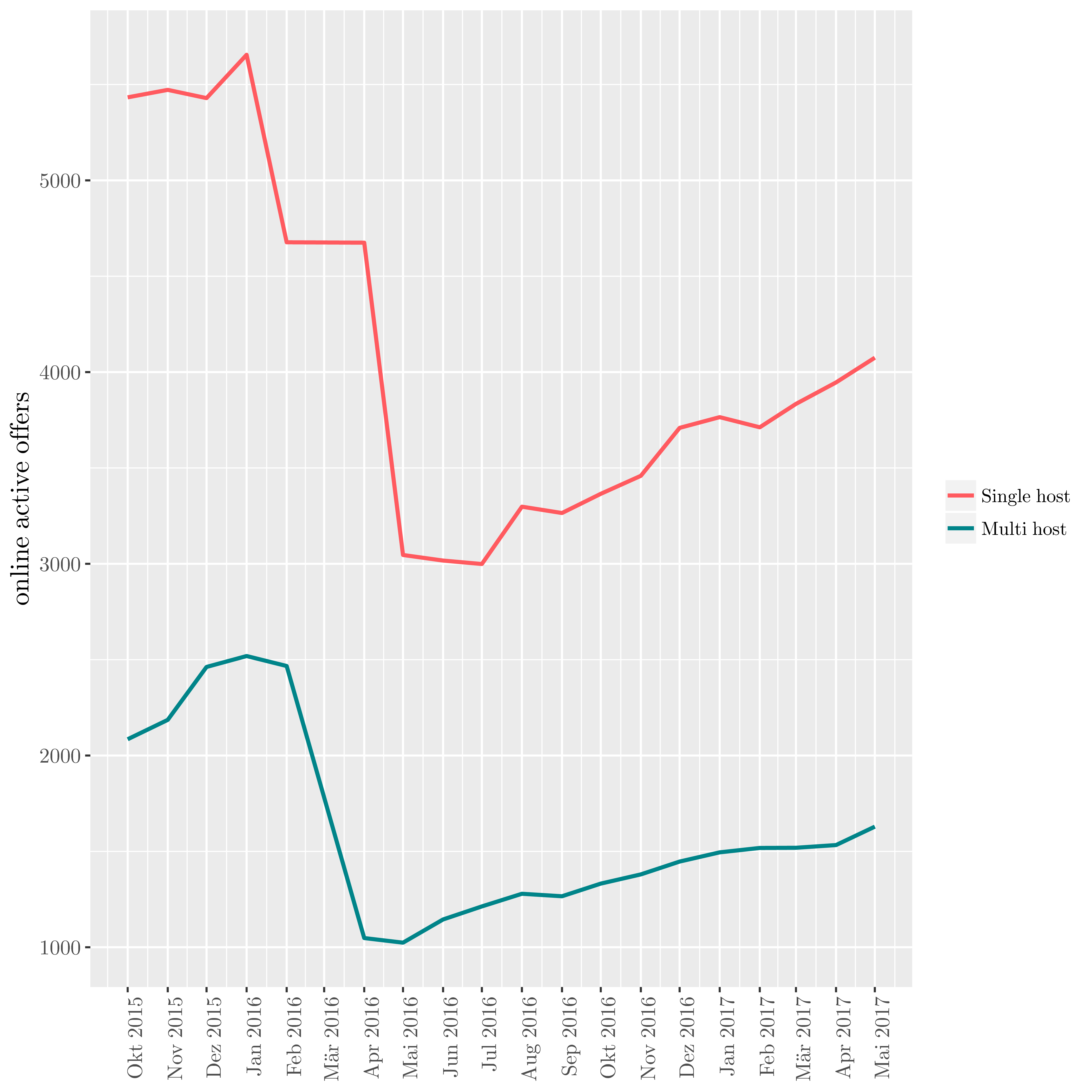
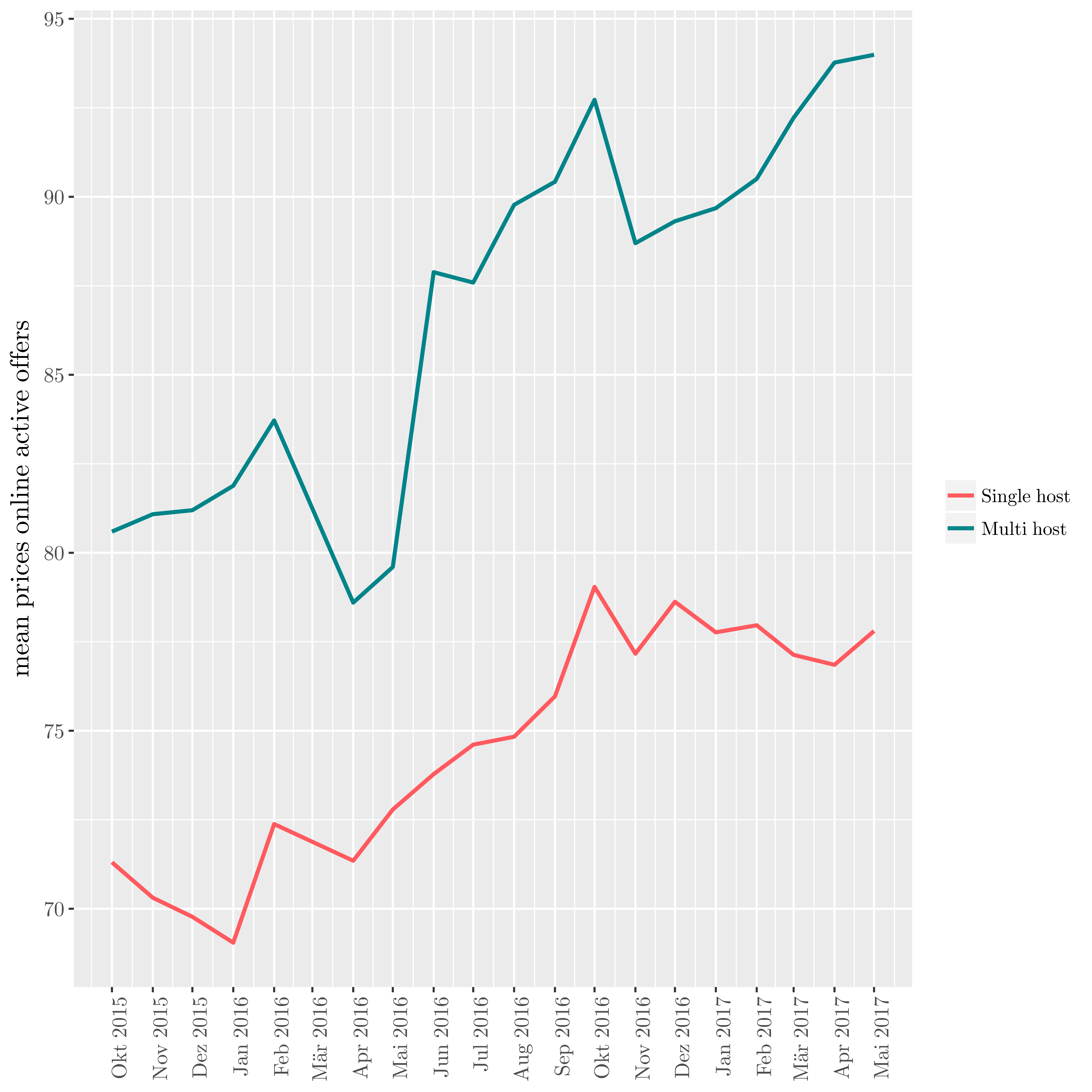
Since may 2016, the renting of full appartments is strictly regulated in Berlin : it requires an authorization from the city Authorities, In 2016, only 58 authorizations have been delivered by the city for 800 applications.
On the chart below, we see the effect of this regulation : the numbers of listings drops, then rise again, with a similar trend for the price.
see Airbnb Regulation: How is New Legislation Impacting the Growth of Short-Term Rentals? for more details.
| Evolution of active listings in Berlin |
|---|
 |
| Evolution of prices |
|---|
 |
Then, looking at the localisation as of may 2017 :
| Localization of active offers in Berlin |
|---|
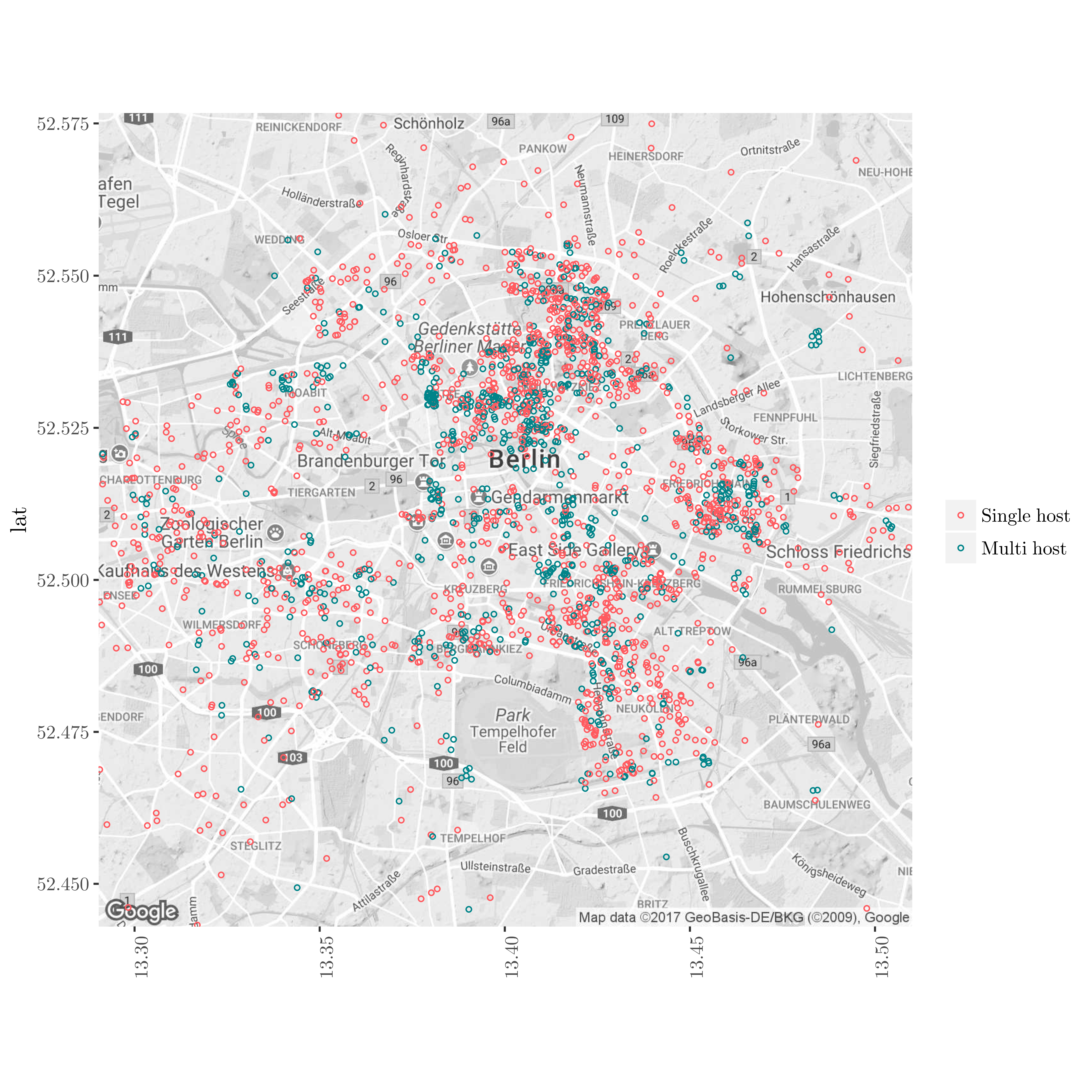 |
We observe three clusters for the multihost listings in Berlin :
- In Mitte,
- In Friedrichshain,
- In Neukoeln.
One of the consequence of the spread of such a disruptive platform is a shortage of affordable housing for the locals. InsideAirBnB, an online activist organization, regulary scraps the entire AirBnB offers for a selection of cities, including Berlin.
Using those data, we can identify professional hosts that potentially break the local regulation.
Problem Statement
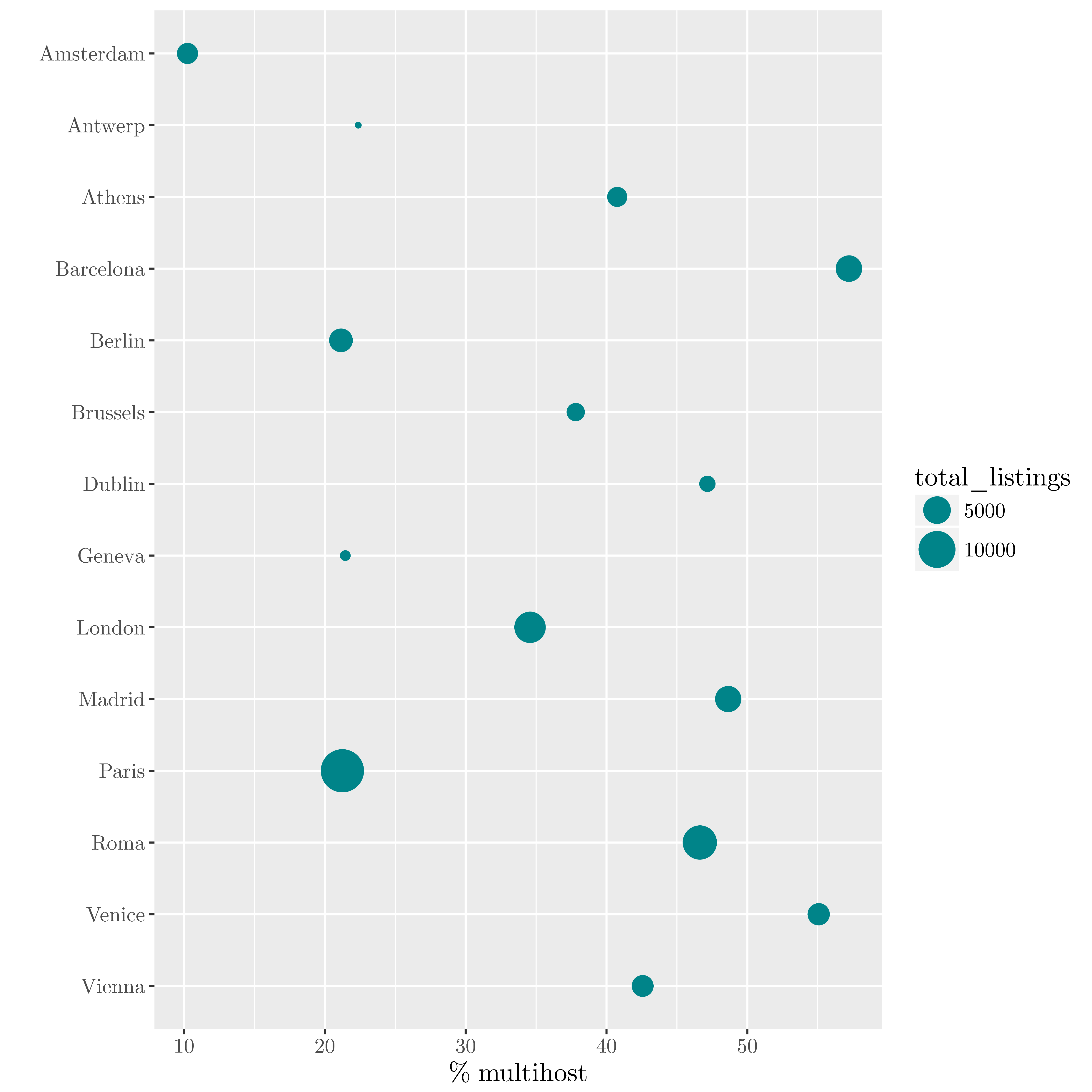
Using those data, we can determine which features characterize the best professional hosts (aka multihosts), ie hosts with more than one active listing.
| Ratio of multihost per city |
|---|
 |
With those selected features, we then build classification models and select the best to identify the professionals.
This model should identify at leadt 90% of the full appartments managed by a professionals.
To solve this problem, we proceed in the following steps :
- filter the dataset on the appartments (i.e full appartments) likely to be offered by professionals,
- process the raw listing provided by InsideAirBnB, the reviews text and appartments pictures,
- convert those data into usable features,
- identify the best features,
- run different classification models
- select the best one.
Metrics
In our context, the aim is to minimize the cost of investigating potential law breakers. In other words, the model should classify the multihost with the lowest False Positive rate (listings classified as multihost, but single host in reality).
To evaluate the quality of our classification model, we will use the standard metrics :
- recall (to evaluate the FPR)
- F1 Score (to get an overall metrics of the classifier)
Definition of the recall (or sensitivity or true positive rate - TPR):
\[recall = $\frac{\sum\ \text{True Positive}}{\sum\ \text{True Positive}+ \sum\ \text{False Negative}}$\]Definition of the F1-score :
\[F1-score = $\frac{2\times{True Positive}}{2\times\text{True Positive}+\text{False Positive}+\text{False Negative}}$\]II. Analysis
Data Exploration
The dataset has been built via the web scraping of the AirBnB website, thus we can considere this is a partial dump of the original database. Formatted as a text file, there are around 100 features available per appartment : price, availability for the next days, picture of the appartment, number of reviews, coordinates, list of offered amenities, etc..
The dataset consists in four tables : the listings informations, the text of the reviews, the timestamp of the reviews and the booking calendar day per day for the next 365 days.
We will use the first three items to build our model.
Regarding the listing informations table,the main table with 95 features, here is a short summary :
| Distribution of missing features in the main table |
|---|
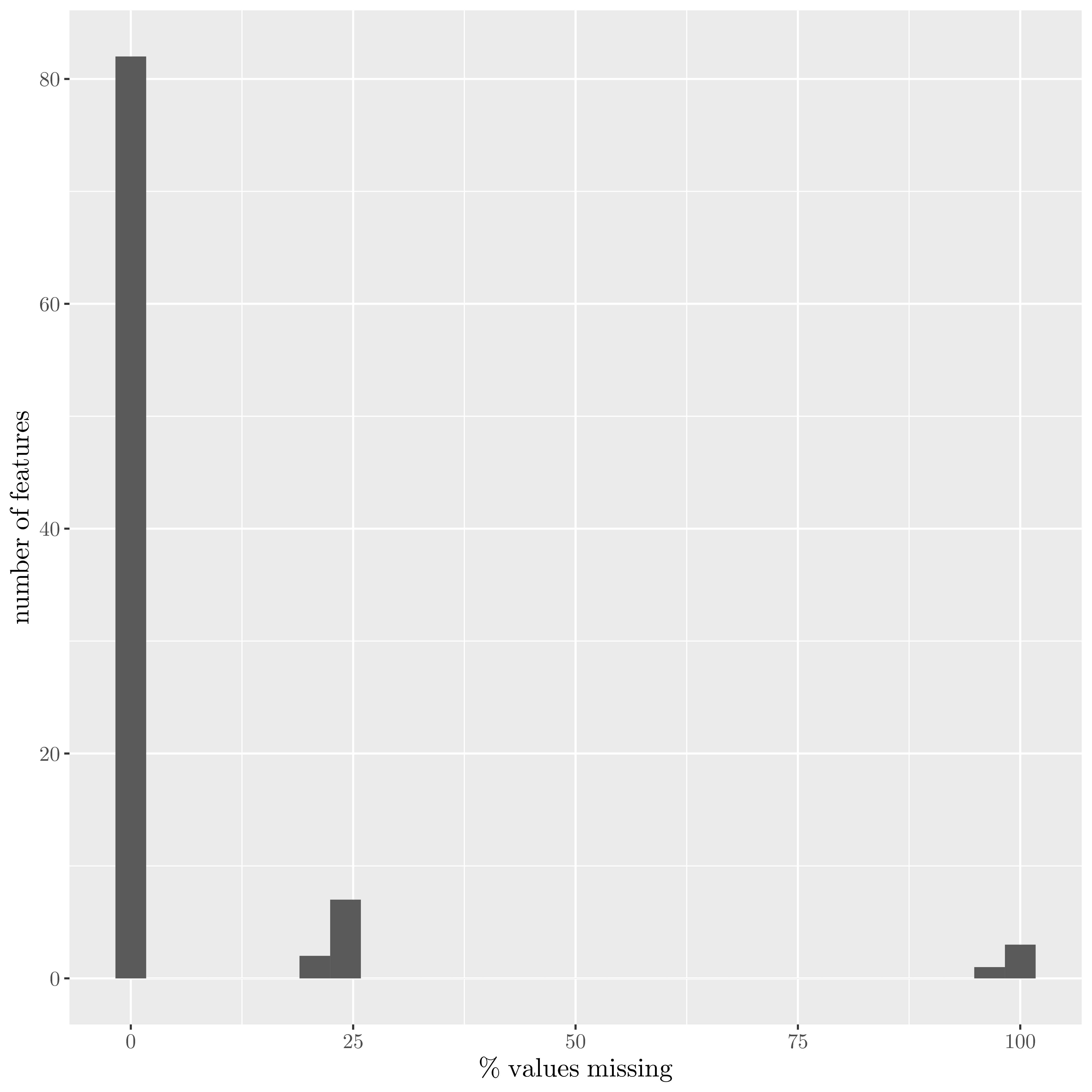 |
As we can see, most of the information are present.
In order to analyse the data, we first eliminate the listing that have no availability at all, meaning the host does not rent it. Unfortunately, we do not have the effective booking information (booking history, amount charged) for each appartment, but we can approximate them via the availability planning.
Then, we have to remove the ‘zombie’ host, online listing that are not active anymore. To proceed, we drop the listing for which the last review is older than two months and the availability for the next 30 days is zero :
Example for Berlin :
| room_type | total_listing | % reviewed | % active |
|---|---|---|---|
| Entire home/apt | 10285 | 80.83 | 30.85 |
| Private room | 10011 | 76.65 | 28.1 |
| Shared room | 280 | 69.29 | 30.42 |
When all data are combined, we get a list of active listings for 14 european capitals with 56879 rows and 411 columns.
Exploratory Visualization
Looking at the dataset, we can see the distribution of appartments per multiple ownership :
| Listing per hosts |
|---|
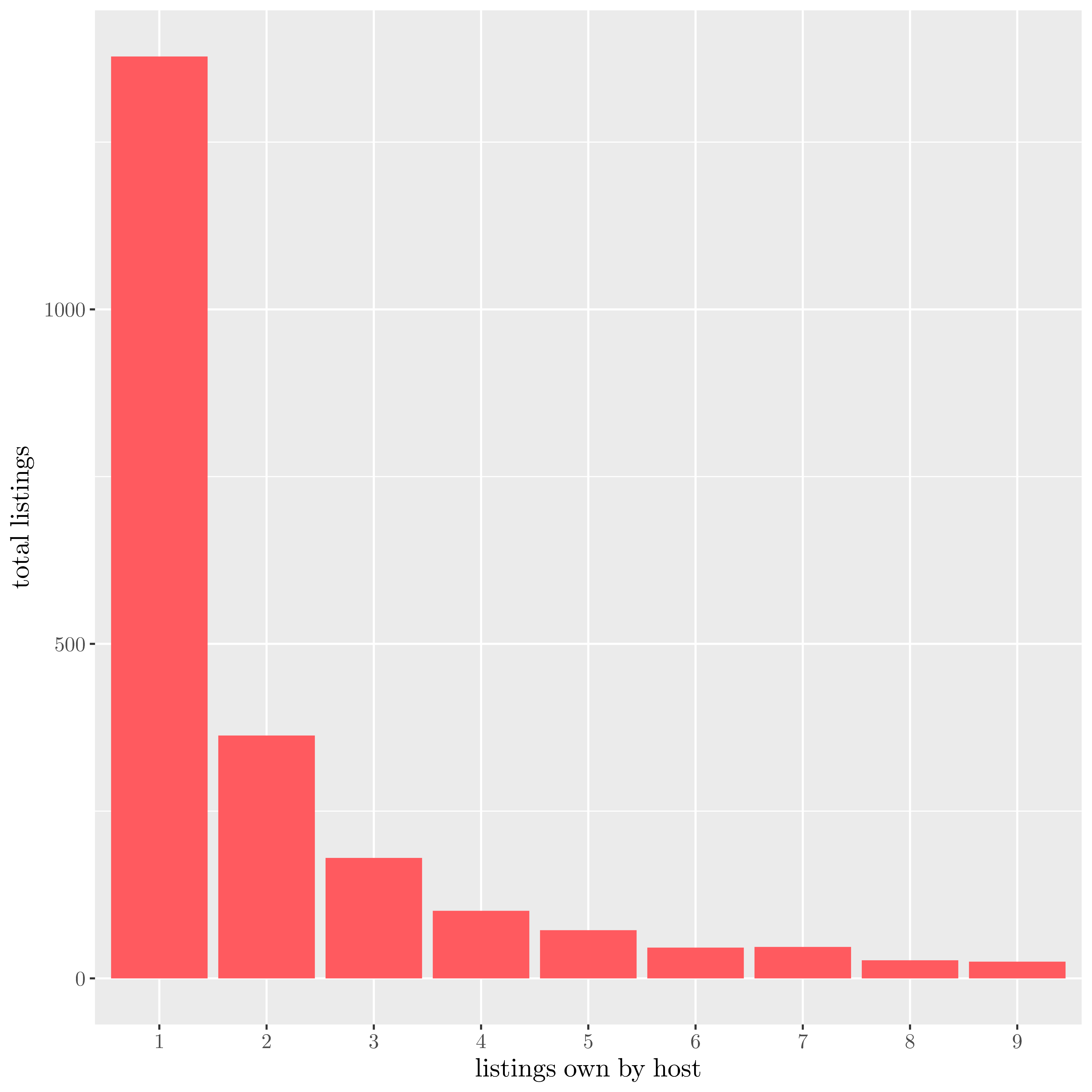 |
There are around one third of active listing that are offered by an host who owns more than one listing. Those are our target population, i.e professionals renting full appartments.
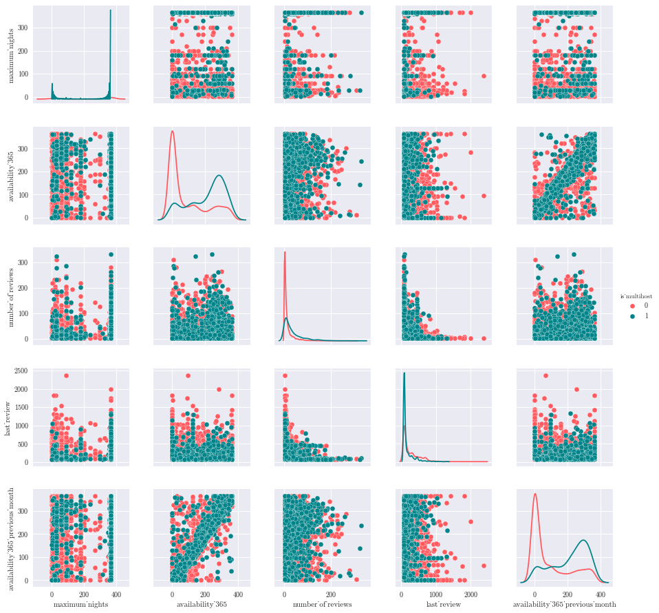
| Number of reviews per listings rented |
|---|
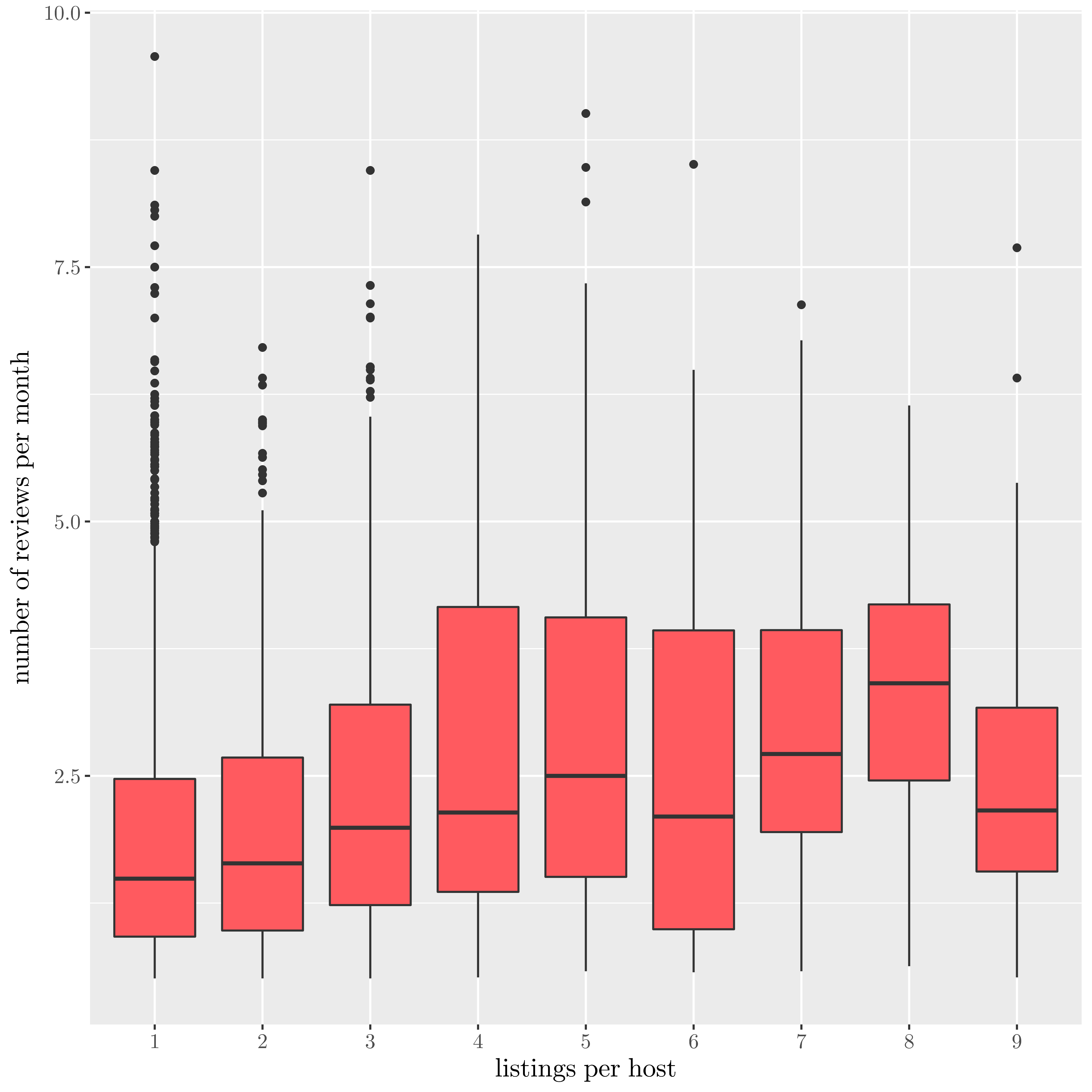 |
| Availability per listings rented |
|---|
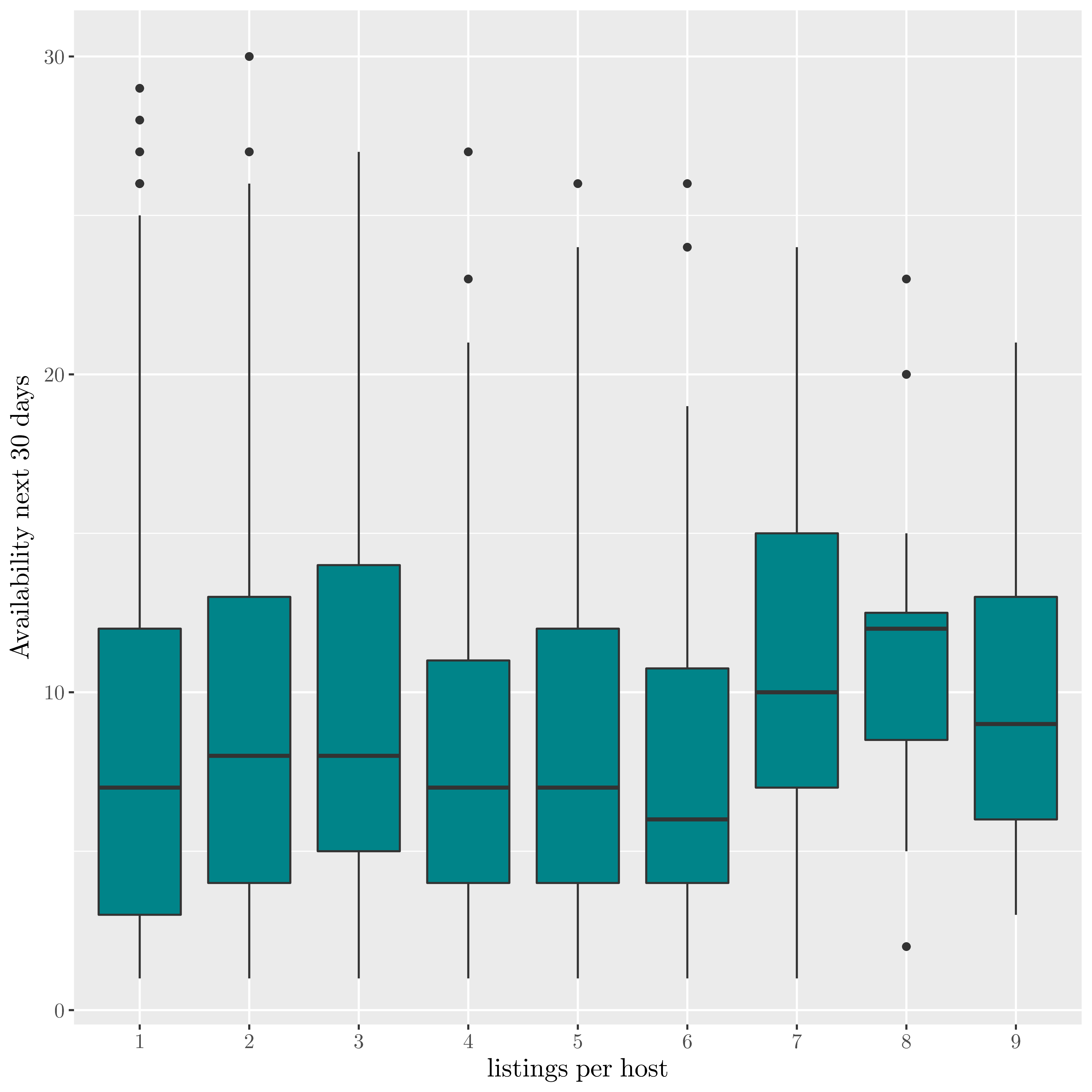 |
The above charts show that professional hosts have an higher number of reviews, but also an higher availability.
| Reviews per language |
|---|
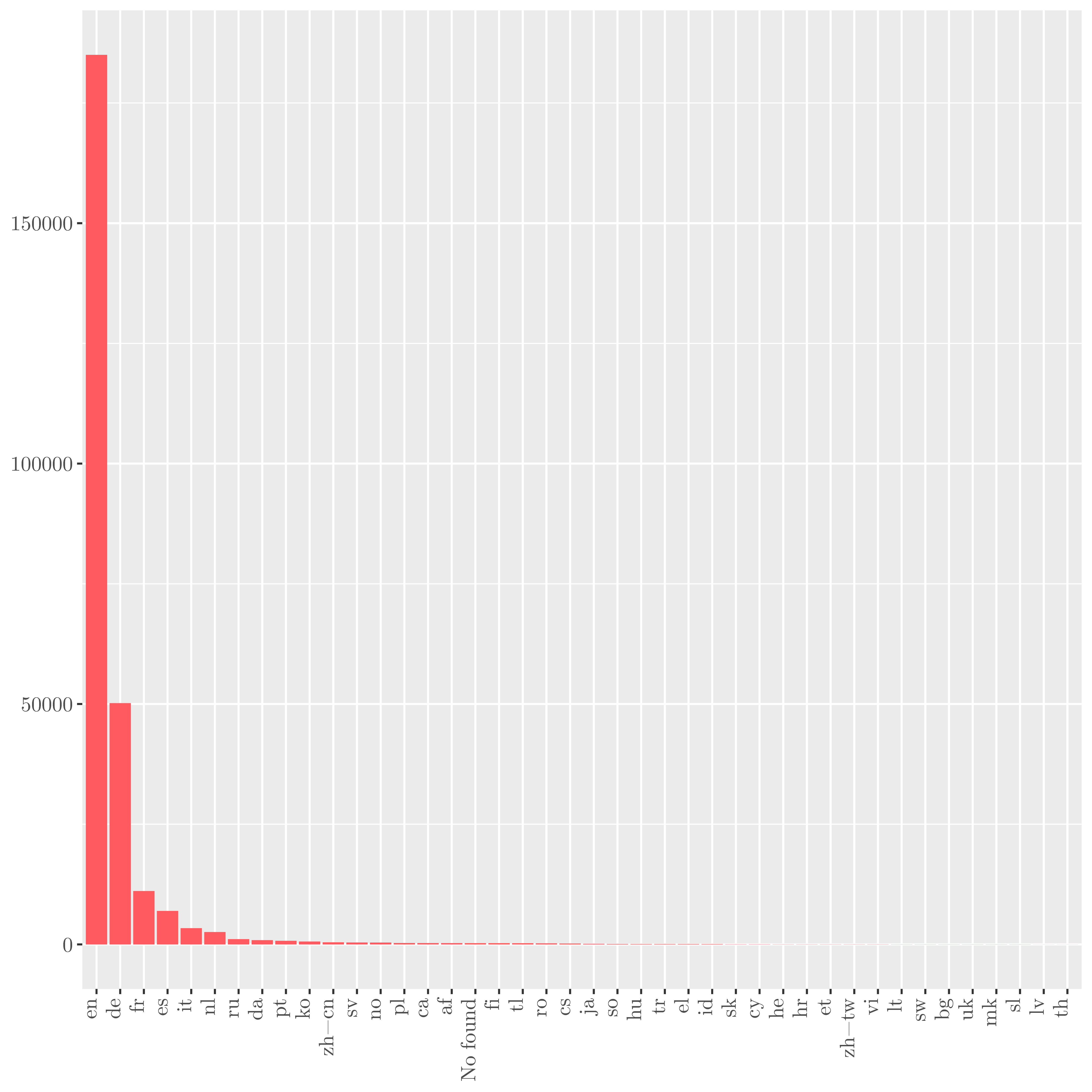 |
English is the overwhelming language for reviews, we will focus then on it for the further text analysis.
Algorithms and Techniques
We implement three different classification algorithms :
a standard logistic regression to be used as a benchmark :
-
Pros : –The fitted model can be formatted as probabilities, which eases its understanding, and Confidence Intervals can be computed. –When the features are lineary separable and are limited, it tends to perform pretty well. –it can be updated with additional training data without hassle.
-
Cons : –if the features are not lineary separable, then it might not be the best approach. –it does not handle well categorical features. oes not handle the multiclass well. –it suffers when there is multicollinearity amongst the features.
a decision tree based algorithm : Xtra Gradient Boosting (XGBoost) Classifier :
- Pros : –does not require much feature engineering nor hyper-parameters tuning. On top of that it is fast.
- Cons : –it tends to overfit on the training set, but can be controlled via the learning rate and tree depth parameters.
Neural Nets based algorithm with a binary classifier using the Keras wrapper with a Tensorflow backend.
- Pros : –They can overperform other classifier with enough data and well designed layers.
- Cons : –require lots of computing power (GPU), slow on regular CPU.
A Support vector machine approach has been excluded due to its heavy hyper parameter tuning.
As the data are weakly correlated with our target, we use a lot of features, and check if some interesting combinations of them can improve the model. The XGB algorithm has the advantage to select itself the best features, and so does the neural network.
Benchmark
In this section, you will need to provide a clearly defined benchmark result or threshold for comparing across performances obtained by your solution. The reasoning behind the benchmark (in the case where it is not an established result) should be discussed. Questions to ask yourself when writing this section:
- Has some result or value been provided that acts as a benchmark for measuring performance?
- Is it clear how this result or value was obtained (whether by data or by hypothesis)?
As we are in the case of a binary classifier, a basic benchmark classifier consist in labeling all the entries as non-professional hosts (66% of the population). We will thus use the Logistic classifier as benchmark and try to get a recall value for the professional higher than 90%.
III. Methodology
Data Preprocessing
-
Main listing The main listing does not requires much preprocessing, if not split the amenities features, which in its original form combine the 100 differents possible amenities (from Dishwasher to children toys) in a single column.
-
Text reviews The text reviews do require a specific processing. We use the detect_lang package from google to identify the language of each review. Then, we select the reviews written in english, stemm the text with the Porter method, vectorize them using the TFIDF (term frequency-inverse document frequency) method on 2 to 3 ngrams, and finally reduce the dimensionality via the Principal Components Analsysis for each city.
Using a multinomial Bayesian classifier, we can get a rough idea of the text reviews weights :
| Value | Single Host | Value | Multihost |
|---|---|---|---|
| -11.87 | - vinni | -6.063 | apart wa |
| -11.87 | emili apart | -6.27 | no comment |
| -11.87 | emili wa | -6.49 | everyth need |
| -11.87 | etienn wa | -6.569 | wa veri |
| -11.87 | imm wa | -6.649 | recommend thi |
| -11.87 | lar wa | -6.695 | wa great |
| -11.87 | lar wa veri | -6.696 | great locat |
| -11.87 | madelin wa | -6.703 | would definit |
| -11.87 | marylis wa | -6.706 | - apart |
| -11.87 | mauric wa | -6.738 | public transport |
| -11.87 | stay emili | -6.782 | - great |
| -11.87 | stay vinni | -6.803 | veri close |
| -11.87 | viliu wa | -6.876 | thi apart |
| -11.87 | vinni great | -6.914 | veri clean |
| -11.87 | vinni place | -6.965 | host wa |
| -11.87 | vinni wa | -6.983 | walk distanc |
| -11.84 | mathia wa | -7.032 | veri help |
| -11.78 | marku wa | -7.042 | wa clean |
| -11.74 | live flat | -7.05 | recommend - |
PCA on text reviews :
| PC1 - PC2 on text reviews |
|---|
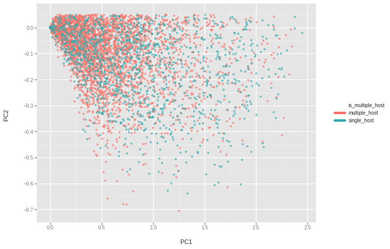 |
The first two PC for each city explain in average 20% of the variance of the Tfidf vectors, which is pretty low compared to the greyscale PC.
TFIDF on 5000 elements, highest weights on PCA with 2 components :
| index | PC1 | PC2 |
|---|---|---|
| apart wa | 0.28 | -0.34 |
| wa veri | 0.2 | -0.2 |
| everyth need | 0.16 | 0.02 |
| would definit | 0.15 | 0.22 |
| recommend thi | 0.15 | 0.36 |
| public transport | 0.13 | -0.075 |
| veri clean | 0.12 | -0.12 |
| veri help | 0.11 | -0.081 |
| great locat | 0.1 | 2.7e-06 |
| wa great | 0.1 | -0.03 |
| stay apart | 0.096 | -0.019 |
| veri nice | 0.094 | -0.05 |
| wa clean | 0.087 | -0.15 |
| flat wa | 0.086 | -0.025 |
| walk distanc | 0.085 | 0.011 |
| thi apart | 0.085 | 0.083 |
| highli recommend | 0.084 | 0.13 |
| minut walk | 0.082 | -0.036 |
| apart veri | 0.081 | -0.018 |
| wa veri help | 0.081 | -0.09 |
- Appartements pictures
For the pictures, after having scrapped the pictures from the Airbnb website (110,020 pictures), we implement the following operations :
- compute the brightness and contrast for each picture,
- compute the 5 top colors via a K-Means clustering on the the RGB features for each picture
- compute a greyscale numpy array for each picture.
- compute a PCA of the greyscale arraus for each city.
Regarding the color clustering, the result are visually not significants :
Colors PCA
Main colors in appartment pictures

Thus, colors clustering has been removed from the features.
The PCA implementation at the level of the city is justified by the limited computing resources. Otherwise, it would have been optimal to run a PCA on both greyscale picture and TFIDF text vectors on the whole dataset.
- Reviews frequency and language ratio
For the review languages, i compute for each listing the ratio of reviews for each language. For the frequency of the reviews, i aggregated the number of reviews in 11 bins : from less than 1 day since the scraping date, to more than 200 days since scraping date
Implementation
The main challenge for this model is the feature selection. With 300 differentes features, and very low correlation with the target (best correlation, maximum nights, scores ${\rho}$ = 0.145 with the multi-host target.)
- Features selection
Now we can check . To select the most relevant features from the listing table to predict the multihosting, i used three differents techniques :
- RandomizedLogisticRegressor,
- KBest features selection based on \({\chi}^2\) and FScore,
- best F-score features from a basic XGBoost classifier.
When those four list are combined, we obtain a list of 100 features.
For this we use the \({\chi}^2\) test on the numerical values :
| \({\chi}^2 best features\) |
|---|
 |
| XGBoost best features |
|---|
 |
| XGB best fclass features |
|---|
 |
Refinement
I used the different combination of features :
- with the RandomizedLogisticRegressor features only,
- with the 20 \({\chi}^2\) best Features,
- with the 20 F-score best features,
- with the 20 best XGBoost Faeatures,
- with all the features combined.
And applied them on classification models :
- logistics regressor,
- random Forest Classifier,
- XGBoost Classifier
- A Neural Net with a relu activation in input and a sigmoid in output with an adam optimizer.
Rebalancing the dataset
One common challenge faced when implementing a classifier is the unbalance of the dataset.
This is the case here, when looking at the full dataset :
| Full dataset balance (target : is multihost) |
|---|
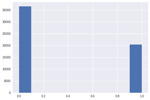 |
It is clear that the model would tend to generate a better recall on the single hosts rather the multihosts.
Thus, before applying the train/test split, i first rebalanced the original dataset (1/3 multihost vs 2/3 single host) to get a 50/50 distribution using the solution provided here
Training and testing set
I used a standard 80%-20% ratio to split the original dataset.
Hyper parameter tuning
XGBoost
For the XGBoost classifier, i used the GridSearch method from scikit-learn combined with a 5 Folds Cross-Validation to extract the best parameters. Here is an overview of the parameters and theirs value i combined :
| parameter | values |
|---|---|
| max_depth | [5,9,12] |
| min_child_weight | [1,2,5] |
| learning_rate | [0.01,0.1] |
| gamma | [0.0,0.1,1] |
| n_estimators | [100,200,500] |
Keras Neural net
layers parameters :
| parameter | values |
|---|---|
| input layer size | [23,64,128,512] |
| input layer activation function | relu,tanh |
| dropout rate (all layers) | [0.2,0.5,0.8] |
| hidden layer activation | relu,tanh |
| output layer activation | sigmoid |
optimizers :
| name | values |
|---|---|
| adam | standard, lr=0.0001 |
| RMSProp | standard, lr=0.0001 |
IV. Results
Model Evaluation and Validation
Using a standard Logistic Regressor on the features provided by the RandomizedLogisticRegressor, we can reach an accuracy of 76%, with a recall of 77%. Lowest results were provided by the Random Forest without tuning, and the Keras Neural net got the same result as the logistics regressor.
It is finally the XGBoost Classifier that got both 80% in accuracy and recall.
With a cross-validation of the training set on 5 folds on a 12231 samples (training set) and 8154 testing samples, we get the following results :
Recall: 0.79% (+/- 0.02)
confusion matrix on the testing set :
| / | single host | multihost |
|---|---|---|
| single host | 3216 | 886 |
| multihost | 829 | 3223 |
classification matrix on the testing set :
| / | precision | recall | f1-score | support |
|---|---|---|---|---|
| single host | 0.80 | 0.78 | 0.79 | 4102 |
| multi host | 0.78 | 0.80 | 0.79 | 4052 |
| avg / total | 0.79 | 0.79 | 0.79 | 8154 |
The fact i used cross-validation and evaluate the model on the testing set after a random balanced sampling makes us confident of the reliability of the result.
ROC Curve for the XGBoost Classifier :
| ROC curve for XGB model |
|---|
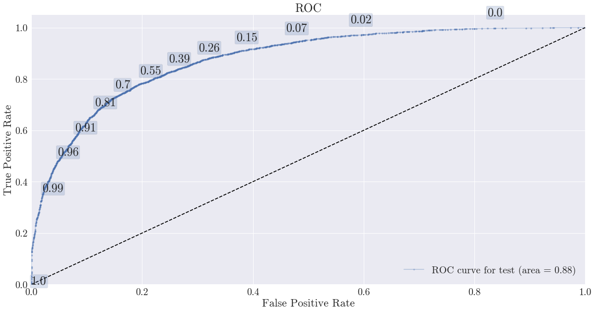 |
Justification
Though the XGB model outperforms the benchmark (Logistics Regressor), it is still does not reach our 90% recall objectif, making it hardly production-grade. We could raise the standard 0.5 probability threshold to 0.7 and get a better recall.
V. Conclusion
Free-Form Visualization
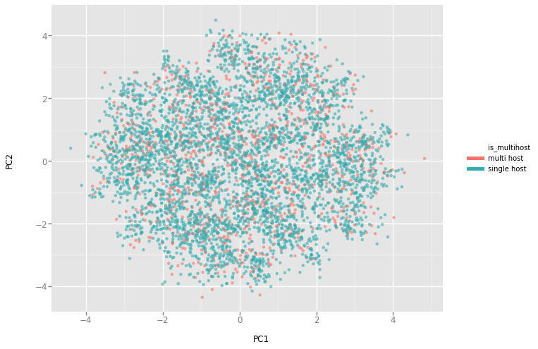
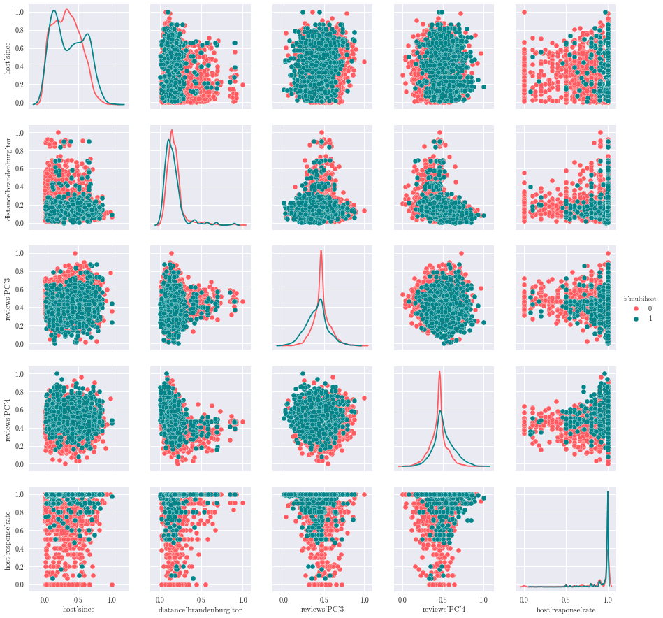
When looking at the first 2 PC of the entire features set PCA :
| PC1 vs PC2 all features on 5000 random listings |
|---|
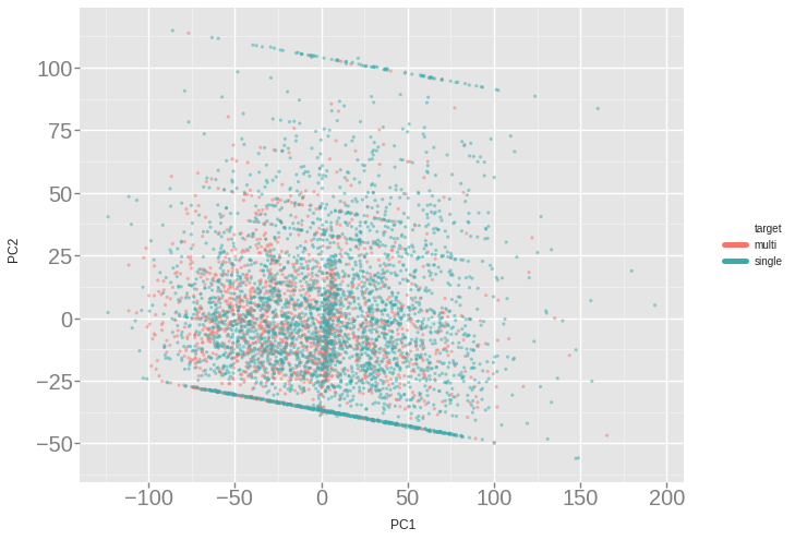 |
From this chart, it is obvious that the two categories are hardly separable. We can also notice the city pattern, characterized by the latitude factor, as listing form parallel line.
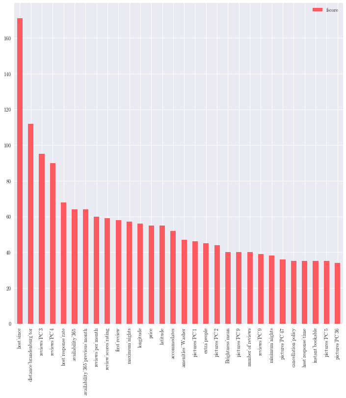
Finally, we can have a look at which features have strong relationship with multihosting :
| Top 10 feature for the XGB Classifier |
|---|
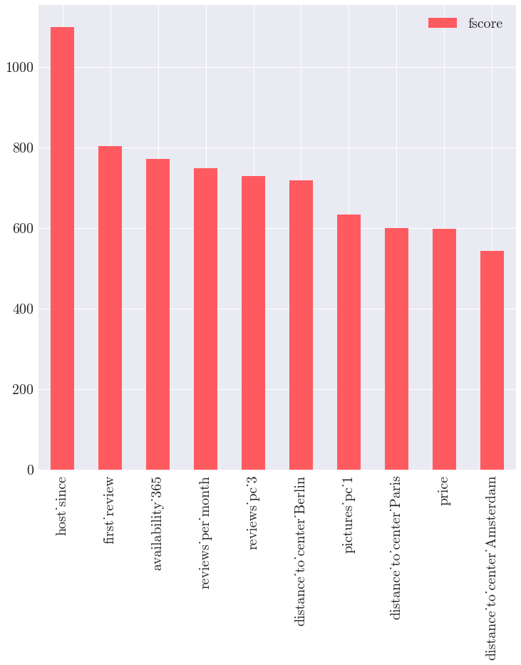 |
Fscore sums up how many times each feature is split on during the training. Thus we do not have insight whether it increae or decrease the multihosting target, but gives an idea how important the feature is in the model :
- Here, the “age” of the guest ( “host since”, “first review” ) seems to significantly weight.
- The listing occupancy, characterized by “frequency of review”, “availability_365”
- Finally, the distance to city center has a influence on the model.
Reflection
The objective was ambitious and the data available have required more work than the modeling phase. When i first used the data for Berlin only, the size of the dataset was not large enough to get stable recall values on the dataset. I then had to extend the scope to thirteen european cities. Though, the recall obtain (80% at best) is not satisfying.
Morevoer, I did put heavy expectation on the neural net, but after hundreds of iteration the model stuck on the validation recall of 76%, i.e. as good as a basic logistics regression.
There is a major flaw in my project : the definition of professional, i.e multihost is per se not accurate ; one professional might offer only one listing on Airbnb, or use two differents identities to rent its appartments.
As too often in such project, the data gathering and wrangling took more than 80% of the overall time. Building a pipeline for retrieve and process the data for the thirteen cities was a funny, though slow, thing to implement.
The most challenging, but also interesting part was the keras neural net to optimize. I could not figure out why the net did not break the 76% recall threshold. My guess is that the dimension of the dataset is not well sized : too many features for too few entries. I tried with a limited number of features (13), but still the performance did not match our logistic regressor benchmark.

Finally, i would compare building a machine learning model to the art of fishing : you first check the state of the sea, put your fishing lines, wait, check, put the lines somewere else until fishes come. In a word : it takes patience and perseverance.
Improvement
If my time was not constrained, i would add more features : profile pictures of the guest, define a list of touristic/interest location per city and compute the distance to it.
An other approach could be to implement three parallel classifiers :
- one on the basic features,
- on the text reviews using LSTM-based neural net classifier,
- and one using a Conv2D-based neural net classifier on the appartment picture.
And combine them using the stacking technique.
I used the tpot python package to identify the best model possible (excluding the deep learning option), and the best proposal was the XGBoost. As the categories are definitively not lineary separable, i would put more emphasis on a SVM classifier with a RBF kernel, which requires lots of hyper-parameter tuning.
Share